Part C: Core techniques
Zero-shot, few-shot, and many-shot
Zero-shot means instructions only. Few-shot means adding a handful of solved examples (the model infers the pattern from them; this ability is called in-context learning). Many-shot means dozens to hundreds of examples, which long context windows now allow; Agarwal et al. ("Many-Shot In-Context Learning", 2024) report significant gains over few-shot across many tasks, and note that inference cost grows linearly with the number of examples. Examples are not free, so measure what they cost first.
"""Zero-, few-, and many-shot: what examples cost in tokens, and how informative each selection is."""
from supportdesk.data import load_tickets

from examples.m04_eval import copy_backend, run_eval, wilson
from examples.m04_prompts import ExampleSelector, arrange, count_prompt_tokens, load_prompt

dev = load_tickets("dev")
query = {t.id: t for t in dev}["T-1001"]
selector = ExampleSelector(dev)
v3 = load_prompt("v3")

print("Prompt size for T-1001 with v3 (o200k_base estimate)")
for k in (0, 3, 6, 12, 24, 47):
    messages = v3.render(query, arrange(selector.similar(query, k)))
    print(f"  k={k:>2}  input tokens {count_prompt_tokens(messages):>5}")

print("\nCopy-the-examples stand-in (NOT a model): category accuracy on dev, n=48")
for shots, k, seed in [("random", 6, 0), ("random", 6, 1), ("random", 6, 2), ("random", 6, 3), ("random", 6, 4),
                       ("similar", 1, 0), ("similar", 6, 0), ("balanced", 6, 0)]:
    run = run_eval(copy_backend(), "v3", "dev", shots, k, backend="copy", seed=seed)
    ok = sum(run.correct("category"))
    lo, hi = wilson(ok, len(run.records))
    print(f"  {shots:<9} k={k} seed={seed}  {ok:>2}/48  acc {ok / 48:.3f}  95% CI [{lo:.3f}, {hi:.3f}]")
Code explained
- In simple words: first measure how big the prompt gets as you add examples; then measure how informative different example sets are, using a stand-in that can only copy the examples' labels.
- What happens: the first loop renders T-1001 with v3 and 0 to 47 similar examples (47 is every other dev ticket: many-shot for this dataset). The second loop runs the whole dev set through the copy stand-in with random examples under five seeds, one similar example, six similar examples, and a balanced set of six.
- Comes out: each example adds about 63 tokens; all 47 make the prompt 11 times larger than zero-shot. The copy stand-in is not a model, but its score is real and it answers a real question: if the model did nothing but follow the examples, how often would the examples point to the right category? Random examples point the wrong way almost always (0.083 to 0.229 across seeds; the spread across seeds alone is 4 to 11 correct, which is how much example choice can move a score). Part of why random is below chance: leave-one-out removes the query's own class from the pool once. One similar example points the right way 28/48 times. Six similar examples do worse (22/48) because the majority of six neighbors is often a common category such as billing. The balanced set ties the one-nearest result exactly: with one example per category every label ties, and the tie goes to the nearest example, so it reduces to the same choice.
Prompt size for T-1001 with v3 (o200k_base estimate)
  k= 0  input tokens   295
  k= 3  input tokens   504
  k= 6  input tokens   690
  k=12  input tokens  1069
  k=24  input tokens  1864
  k=47  input tokens  3257

Copy-the-examples stand-in (NOT a model): category accuracy on dev, n=48
  random    k=6 seed=0   4/48  acc 0.083  95% CI [0.033, 0.196]
  random    k=6 seed=1  10/48  acc 0.208  95% CI [0.117, 0.343]
  random    k=6 seed=2   6/48  acc 0.125  95% CI [0.059, 0.247]
  random    k=6 seed=3  11/48  acc 0.229  95% CI [0.133, 0.365]
  random    k=6 seed=4   5/48  acc 0.104  95% CI [0.045, 0.222]
  similar   k=1 seed=0  28/48  acc 0.583  95% CI [0.443, 0.712]
  similar   k=6 seed=0  22/48  acc 0.458  95% CI [0.326, 0.597]
  balanced  k=6 seed=0  28/48  acc 0.583  95% CI [0.443, 0.712]
What about a real model? Min et al. ("Rethinking the Role of Demonstrations", 2022) found that for classification, the label space, the input distribution, and the format shown by the examples mattered more than whether each example's label was correct. That is why the examples in this module are always real tickets with the exact output format. Run the harness with --backend llm and --shots none, random, similar, and balanced to see which matters for your model.
| Situation | Use this | Why |
|---|---|---|
| Labels are self-explanatory, strong model, tight budget | Zero-shot with clear definitions | Cheapest; definitions carry most of the signal |
| Model confuses neighboring labels (how_to vs bug) | Few-shot, similar examples, most similar last | Shows the boundary right where the ticket sits |
| Label distribution is skewed | Balanced few-shot | Stops the examples from voting for the common class |
| Many labels or a subtle house style, long-context model | Many-shot with a cached block | Gains can continue past a few examples; caching limits the cost |
| No labeled pool yet | Zero-shot, then label real traffic | You cannot select examples you do not have |
Selection, order, and label distribution
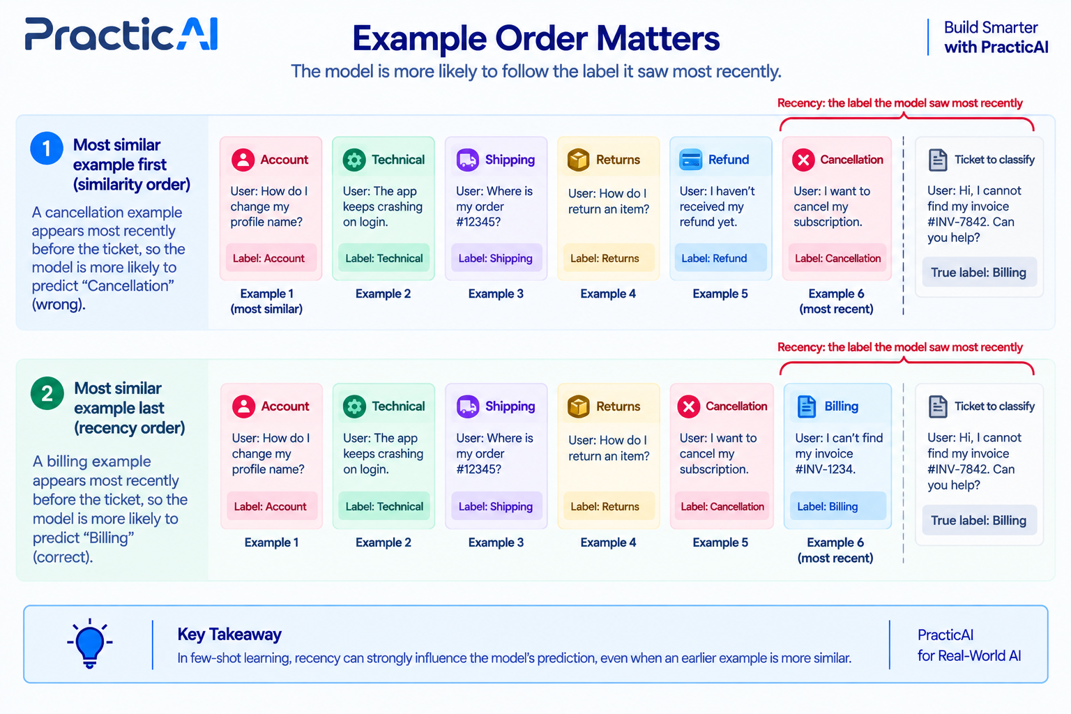
Zhao et al. ("Calibrate Before Use", 2021) showed that few-shot answers drift toward labels that are frequent among the examples (majority label bias) and toward the label of the last examples (recency bias). Lu et al. ("Fantastically Ordered Prompts", 2022) showed that example order alone can swing accuracy widely. You cannot measure a real model's bias here without a key, but you can measure exactly what your prompt feeds it: which labels the examples show, and which label sits last.
"""Label distribution and order of few-shot sets: which label sits last, right before the ticket?"""
from collections import Counter

from supportdesk.data import CATEGORIES, load_tickets

from examples.m04_prompts import ExampleSelector, arrange, gold_labels, label_counts

dev = load_tickets("dev")
by_id = {t.id: t for t in dev}
selector = ExampleSelector(dev)

for ticket_id in ("T-1001", "T-1034"):
    q = by_id[ticket_id]
    print(f"{ticket_id} gold={q.gold['category']}  {q.subject}")
    for name, examples in [("similar k=6", selector.similar(q, 6)), ("balanced k=6", selector.balanced(q))]:
        counts = dict(label_counts(examples))
        first = arrange(examples, "first")[-1].gold["category"]
        last = arrange(examples, "last")[-1].gold["category"]
        print(f"  {name:<13} labels={counts}")
        print(f"  {'':<13} last label if most similar placed first: {first:<16} placed last: {last}")

print("\nAcross all 48 dev tickets (similar k=6):")
gold_is_last = {"first": 0, "last": 0}
majority_hits = 0
shown = Counter()
for q in dev:
    examples = selector.similar(q, 6)
    shown.update(label_counts(examples))
    majority_hits += label_counts(examples).most_common(1)[0][0] == q.gold["category"]
    for order in gold_is_last:
        gold_is_last[order] += arrange(examples, order)[-1].gold["category"] == q.gold["category"]
print(f"  gold label is the LAST example: most-similar-first {gold_is_last['first']}/48, "
      f"most-similar-last {gold_is_last['last']}/48")
print(f"  majority label of the set equals gold: {majority_hits}/48")
print(f"  labels shown in total: {dict(shown.most_common())}")

print("\nBalanced set in a FIXED category order (the order CATEGORIES is declared in):")
fixed_last = Counter()
for q in dev:
    examples = selector.balanced(q)
    fixed = sorted(examples, key=lambda t: CATEGORIES.index(t.gold["category"]))
    fixed_last[fixed[-1].gold["category"]] += 1
print(f"  last label across 48 prompts: {dict(fixed_last)}")
print(f"  needs_human in similar-6 sets, share true: "
      f"{sum(gold_labels(t)['needs_human'] for q in dev for t in selector.similar(q, 6)) / (48 * 6):.2f}")
Code explained
- In simple words: inspect the example sets for two tickets, then count across the dev set which label ends up in the last slot and which labels are shown most.
- What happens: for T-1001 (English billing) and T-1034 (Japanese cancellation) it prints the label counts of the similar and balanced sets and the last label under both orders. Then, over all 48 dev tickets, it counts how often the gold label is last, how often the set's majority label is the gold label, and the total labels shown. Finally it builds balanced sets in a fixed category order, the kind of order you get from a hand-written list.
- Comes out: four things worth acting on.
- Order changes the last label: with most-similar-first, the gold category sits in the last slot 6/48 times; with most-similar-last, 28/48 times. If recency bias exists in your model, the second order points it the right way.
- The fixed category order puts
feature_requestlast in all 48 prompts. A recency bias would then push every ticket towardfeature_request. Sort by similarity or shuffle per ticket; never use a fixed label order. - Similarity selection skews the label distribution: billing is shown 94 times, feature_request 11. Billing tickets share generic words like "plan" and "team" with many tickets. Balanced selection fixes this by construction.
- Word-overlap similarity fails across languages: the Japanese cancellation ticket gets four billing examples, because its only English word is "Team". Module 7 introduces embeddings, which handle this far better.
Specificity over politeness
Models do not need to be asked nicely; they need to be told precisely. Politeness costs tokens and carries no information. Vague words ("really bad", "might be") force the model to guess where your boundary is, and different models guess differently.
"""Politeness vs specificity, negative vs positive: what each wording costs and what it tells the model."""
from supportdesk.tokens import count_tokens

from examples.m04_prompts import lint_prompt

PAIRS = {
    "polite and vague": ("Could you please kindly take a careful look at this ticket and let me know what you "
                         "think the priority might be? Thank you so much, I really appreciate it!"),
    "specific": ("Set priority to urgent only when many users are blocked right now or there is a security "
                 "risk right now."),
    "negative": ("Don't mark tickets urgent unless it's really bad. Do not use high for simple questions. "
                 "Never pick low for bugs. Don't overthink it."),
    "positive": ("Use urgent when many users are blocked now. Use high when one user is blocked or money was "
                 "charged wrongly. Use low for questions and ideas."),
}
for name, text in PAIRS.items():
    kinds = [f.kind for f in lint_prompt(text)]
    print(f"{name:<17} {count_tokens(text):>3} tokens  lint: {kinds or 'clean'}")
Code explained
- In simple words: four ways to say what priority means, measured in tokens and checked with the lint.
- What happens: each string is counted with the o200k_base tokenizer and run through
lint_prompt. - Comes out: the polite, vague request is the longest (33 tokens) and defines nothing. The specific rule is shorter (21 tokens) and states a condition someone could check. The negative version gets flagged for heavy negation; the positive version covers three levels in about the same space.
A useful test for specificity: could Maya read the instruction and label the ticket herself, the same way twice? "Use urgent when many users are blocked now" passes. "Don't mark tickets urgent unless it's really bad" fails.
Positive instruction over negative instruction
"Do not use high for simple questions" tells the model one thing that is wrong and nothing that is right. "Use low for questions and ideas" tells it where the ticket should go. Negative instructions still have a place for hard limits ("never reveal another customer's data"), but pair each with the positive action ("if asked, say you can only discuss this account"). The lint flags a prompt with four or more negations as a nudge to rewrite, not as an error.
| Situation | Use this | Why |
|---|---|---|
| Describing what a label means | Positive definition with a checkable condition | Gives the model a target, not just a fence |
| A hard safety or policy limit | Negative rule plus the positive alternative | The limit is explicit and the model knows what to do instead |
| Fixing one recurring mistake | Add a definition or an example that covers the case | A bare "don't do X" patch tends to accumulate into a negative-heavy prompt |
Decomposition into steps
Decomposition splits a task into smaller calls: first extract facts, then decide. It can help when one call has to do two different kinds of work, and it always costs more calls and tokens. You can measure the cost now; the accuracy effect needs a real model.
"""Decomposition: one triage call vs a two-step chain (extract facts, then label).

The chat function is ScriptedLLM, so this measures plumbing and token cost only,
not whether decomposition makes a real model more accurate. Swap in
supportdesk.llm.chat to measure that on the frozen dev set.
"""
import json

from supportdesk.data import load_tickets
from supportdesk.stand_in import ScriptedLLM

from examples.m04_eval import keyword_triage, last_ticket_text
from examples.m04_prompts import load_prompt, parse_triage, render_ticket

FACTS_SYSTEM = """You read one Brightlane support ticket inside <ticket> tags and extract facts.
Reply with one JSON object with these keys and nothing else:
{"language": "<ISO 639-1 code>", "money_involved": true|false, "users_blocked": "none"|"one"|"many",
 "asks_for": "<the customer's request in at most 12 English words>"}"""

LABEL_SYSTEM = load_prompt("v2").system + "\nYou also get <facts> extracted in an earlier step. Use them."


def facts_responder(messages, kwargs):
    text = last_ticket_text(messages).lower()
    return json.dumps({"language": "en", "money_involved": any(w in text for w in ("charged", "refund", "usd")),
                       "users_blocked": "many" if "anyone" in text else "none", "asks_for": "refund a duplicate charge"})


def label_responder(messages, kwargs):
    return json.dumps(keyword_triage(last_ticket_text(messages)))


ticket = {t.id: t for t in load_tickets("dev")}["T-1001"]

single = ScriptedLLM(responder=label_responder)
one = single(load_prompt("v2").render(ticket))
print(f"single call : calls=1 input_tokens={one.usage.input_tokens} output_tokens={one.usage.output_tokens}")
print(f"  labels {parse_triage(one.text)[0]}")

step1, step2 = ScriptedLLM(responder=facts_responder), ScriptedLLM(responder=label_responder)
facts = step1([{"role": "system", "content": FACTS_SYSTEM}, {"role": "user", "content": render_ticket(ticket)}])
second_user = f"<facts>{facts.text}</facts>\n{render_ticket(ticket)}"
labels = step2([{"role": "system", "content": LABEL_SYSTEM}, {"role": "user", "content": second_user}])
total_in = facts.usage.input_tokens + labels.usage.input_tokens
total_out = facts.usage.output_tokens + labels.usage.output_tokens
print(f"two steps   : calls=2 input_tokens={total_in} output_tokens={total_out}")
print(f"  step 1 facts  {facts.text}")
print(f"  step 2 labels {parse_triage(labels.text)[0]}")
Code explained
- In simple words: measure how confidently TinyLM produces the correct support answer with no persona, an "expert" persona, and a silly persona.
- What happens: for five question and answer pairs taken from the corpus templates, the script sums the log-probability of each answer token given the prefix (0 would mean certain). It repeats this with each persona line in front.
- Comes out: the plain prompt gives the correct answers a mean log-probability of -0.014 (near certain). The expert persona lowers it to -0.273, and even the pirate persona (-0.149) hurts less. For TinyLM, the persona is unfamiliar text that pulls the context away from what it memorized. TinyLM is a 1M-parameter model with no instruction tuning, so read this as the mechanism (a persona is conditioning, not knowledge), not as a prediction for large models.
none            mean log-prob of the correct answer  -0.014   per pair [-0.02, -0.01, -0.02, -0.01, -0.01]
expert persona  mean log-prob of the correct answer  -0.273   per pair [-0.1, -0.08, -1.02, -0.06, -0.1]
wrong persona   mean log-prob of the correct answer  -0.149   per pair [-0.09, -0.09, -0.43, -0.06, -0.07]
| Situation | Use this | Why |
|---|---|---|
| You need a particular tone or register | A short role line plus a concrete style rule | Role sets register; the rule makes it checkable |
| You need domain accuracy | Definitions, examples, or retrieved facts (Module 7) | A persona does not add facts |
| You are tempted by "world-class expert" | Delete it and measure | It costs tokens and, in published tests, does not raise accuracy |